Databases and Data Management for AI
Master vector databases, RAG architectures, and data pipelines for AI applications
Section 1: The Data Foundation of AI
Why Data Architecture Matters for AI
If AI models are the engine, data is the fuel. But not all fuel tanks are created equal. The way you store, organize, and retrieve data fundamentally determines what your AI applications can do and how well they perform.
Traditional applications primarily work with structured data: users, products, transactions, things that fit neatly into tables with defined schemas. AI applications, however, need to work with meaning and semantics. They need to find similar concepts, understand context, and retrieve relevant information even when exact matches don’t exist.
This shift requires a fundamental rethinking of database architecture.
Most production AI systems operate with three complementary data layers: a transactional layer (traditional databases for structured business data), a semantic layer (vector databases for meaning-based retrieval), and a cache layer (fast access for frequently needed data). Understanding when and how to use each layer is crucial for building AI systems that are both powerful and practical.
From Keywords to Concepts
The fundamental shift in AI-powered data retrieval is moving from exact matching to semantic similarity.
Traditional search asks: “Show me documents containing ‘machine learning.’” It relies on exact keyword matches and misses synonyms, related concepts, and different phrasings.
AI-powered search asks: “Show me documents similar to this concept.” It understands meaning and context and finds relevant content even without keyword overlap.
This shift is powered by embeddings, numerical representations of meaning that we can store, compare, and search mathematically. Vector databases are purpose-built for this new paradigm.
Section 2: Traditional Databases in AI Systems
SQL Databases: The Structured Foundation
Despite the emergence of vector databases, traditional SQL databases remain essential in AI systems. They handle the structured data that AI applications still need.
SQL is the right choice for user management and authentication, which requires transactional integrity for user profiles, permissions, and sessions. Consider storing user preferences for personalized AI responses. SQL excels at application state and metadata: conversation history metadata (not the embeddings themselves), document upload records, and AI feature usage tracking. For audit and compliance, SQL captures who accessed what AI feature when, maintains data lineage for AI decisions, and fulfills requirements for regulated industries.
A typical AI chatbot schema stores users with their IDs and emails, conversations linked to users, messages within conversations (where the actual content might live in a vector database), and documents with their processing status and chunk counts. The SQL layer provides the relational structure and transactional guarantees while referencing the semantic content stored elsewhere.
NoSQL Databases: Flexibility for Unstructured Data
NoSQL databases excel at storing the variable, unstructured data common in AI applications.
Use NoSQL for document storage: original documents before chunking, full conversation histories, and flexible schemas as AI features evolve. Use it for session context: temporary user state during AI interactions, prompt templates and variations, and A/B test configurations. Use it for metadata and tags: document categories, tags, custom fields, user-defined attributes for search, and rapidly changing feature flags.
The Hybrid Approach
Most production AI systems use both SQL and NoSQL databases alongside vector databases. SQL handles critical structured data requiring transactions. NoSQL handles flexible document storage and rapid iteration. Vector databases handle semantic search and similarity operations. The key is understanding the strengths of each and designing your architecture accordingly.
Section 3: Vector Databases Deep Dive
What Makes Vector Databases Different
Traditional databases answer the question “give me the exact record with this ID.” Vector databases answer a different question: “give me the records most similar to this one.” That seemingly simple shift requires completely different underlying technology.
When you search a traditional database for a user by ID, the system uses hash tables or B-trees to find the exact record instantly. When you search a vector database for documents similar to a query, the system must compare your query embedding against potentially millions of stored embeddings. Brute-force comparison would be O(n), impossibly slow. So vector databases use clever index structures like HNSW that organize vectors by similarity, enabling approximate nearest neighbor search in O(log n) time.
In AI contexts, a vector is an array of numbers (typically 384 to 1536 dimensions) that represents the meaning of some content. Two vectors that are close together in this high-dimensional space represent similar meanings, even if the original text was completely different.
Vector Similarity Metrics
To find “similar” vectors, we need a mathematical definition of similarity. The three most common metrics are cosine similarity, Euclidean distance, and dot product.
Cosine similarity measures the angle between vectors, ranging from -1 (opposite) to 1 (identical). It’s the most common metric for text embeddings because it ignores magnitude and only considers direction. If two documents are about the same topic but one is longer, their embeddings will point in similar directions even if the magnitudes differ.
Euclidean distance (L2) measures the straight-line distance between vectors. Lower distance means more similar. It’s sensitive to magnitude and often used for image embeddings and spatial data.
Dot product measures alignment and magnitude. Higher values mean more similar. It’s the fastest to compute and works well for normalized vectors.
Vector Indexing Strategies
The magic of vector databases is finding similar vectors quickly among millions or billions of entries. This requires specialized indexing algorithms.
HNSW (Hierarchical Navigable Small World) is the most popular indexing algorithm, used by Pinecone, Weaviate, and others. It builds a multi-layer graph of connections. Top layers have long-range connections for coarse navigation. Bottom layers have short-range connections for fine-grained search. A query starts at the top and navigates down to find nearest neighbors.
HNSW offers fast query times at O(log n), excellent recall for finding true nearest neighbors, and a good balance of speed and accuracy. The trade-off is higher memory usage because it stores the graph structure. Configuration parameters include efConstruction (build-time quality), maxConnections (connections per layer), and ef (query-time search breadth).
IVF (Inverted File Index) divides the vector space into clusters, then searches only relevant clusters. It clusters vectors using k-means or similar algorithms. At query time, it finds the closest cluster centers and searches only within those clusters. IVF offers very fast queries and lower memory usage, but there’s some accuracy loss because it may miss nearest neighbors in other clusters. It’s well-suited for massive scale with billions of vectors.
Choosing an Index
For most applications with millions of vectors, HNSW provides the best balance of speed and accuracy. Use IVF when you need to scale to billions of vectors or memory is constrained. Flat (brute force) search is only practical for small datasets under 10,000 vectors, but provides perfect accuracy.
Major Vector Database Options
Pinecone is a fully managed, cloud-native vector database. It offers zero operations overhead, excellent performance and reliability, a simple API, and built-in filtering and metadata. The considerations are that it’s cloud-only (potential vendor lock-in), pricing scales with usage, and you have less control over infrastructure.
Weaviate is an open-source vector database with rich querying capabilities. It can be self-hosted or cloud-hosted, has built-in vectorization modules, offers powerful filtering and hybrid search, and provides a GraphQL API. The considerations are that it’s more complex to operate and requires infrastructure management if self-hosted.
Chroma is a lightweight, embeddable vector database for developers. It’s easy to get started, runs in-process or client-server mode, has built-in embedding generation, and is great for prototyping. The considerations are that it’s less mature for production scale, has fewer advanced features, and has a smaller community.
pgvector is a PostgreSQL extension adding vector capabilities to your existing database. It uses existing PostgreSQL infrastructure, combines relational and vector data, provides ACID transactions, and offers a familiar SQL interface. The considerations are that it’s not optimized purely for vectors, scaling requires PostgreSQL expertise, and performance may lag specialized solutions at massive scale.
Section 4: RAG Data Architecture
The RAG Pattern Overview
Retrieval-Augmented Generation (RAG) is the most common pattern for building AI applications with your own data. It addresses the core limitation of LLMs: they only know what they were trained on.
When you ask Claude a question about your company’s documentation, this is what happens behind the scenes: your question gets embedded into a vector, that vector gets compared against millions of document chunks, the most similar chunks get retrieved, and they’re stuffed into the prompt alongside your question. Claude answers based on that retrieved context. That’s RAG.
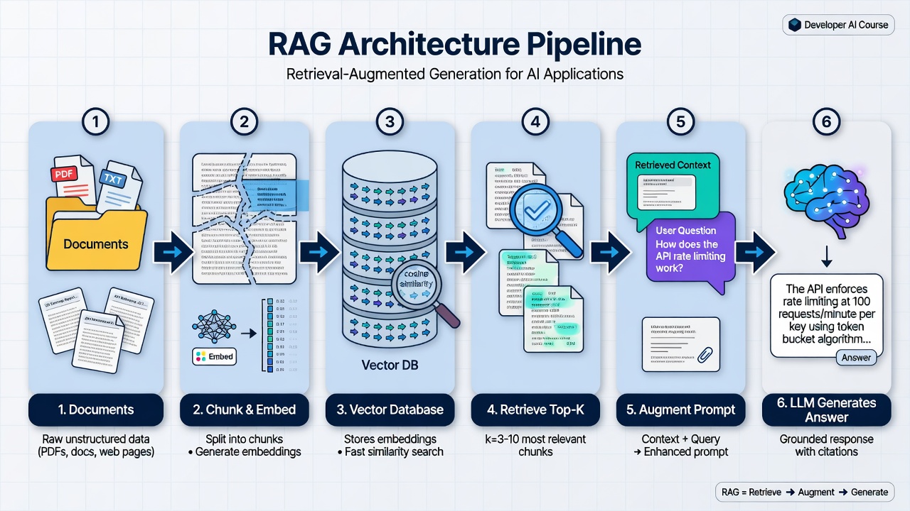
The standard RAG architecture that powers most production systems needing reliable access to private or changing information.
A pattern that combines information retrieval with text generation. First, relevant documents are retrieved using similarity search. Then, these documents are provided as context to an LLM, which generates an answer grounded in the retrieved information. RAG solves the problem of LLMs only knowing their training data by giving them access to your specific knowledge base at query time.
The three stages are indexing (offline), retrieval (query time), and generation (query time). Indexing ingests documents, splits them into chunks, generates embeddings, and stores them in a vector database. Retrieval converts the user question to an embedding, searches for similar chunks, and applies filters and re-ranking. Generation constructs a prompt with retrieved context, sends it to the LLM, and returns the answer.
Chunking Strategies
Chunking is the art of splitting documents into pieces that are meaningful for both retrieval and context provision.
Why chunk? Documents are often too long for single embeddings. Different parts may be relevant to different queries. Embeddings work best on focused, coherent text. LLMs have context window limits.
Chunk size is a critical trade-off. Small chunks (100-200 tokens) retrieve precise information but lose surrounding context. Large chunks (1000+ tokens) preserve context but may include irrelevant information that confuses the model. Most production systems use 500-800 tokens with 50-100 token overlap between chunks.
Fixed-size chunking splits text into fixed character or token counts with overlap. It’s simple and predictable but may split mid-sentence or mid-concept.
Sentence and paragraph chunking splits on natural boundaries and groups to target size. It preserves natural boundaries but produces variable sizes that may be too small or too large.
Recursive chunking splits hierarchically using paragraphs, then sentences, then words until reaching the target size. It balances natural boundaries with size control but has more complex implementation.
Semantic chunking uses embeddings to find natural topic boundaries. When similarity between consecutive sentences drops below a threshold, it indicates a topic change and a good place to split. This respects semantic boundaries but is expensive (requires embedding every sentence) and produces variable sizes.
Chunking Strategy Matters
Choose based on your content type. Technical documentation benefits from recursive chunking that respects structure. Conversational text works well with sentence or paragraph boundaries. Mixed content often does best with fixed-size chunking with overlap as a reliable default. High-quality corpora where accuracy is paramount may justify the cost of semantic chunking.
Metadata and Filtering
Raw vector search isn’t always enough. Metadata enables hybrid approaches that combine semantic similarity with traditional filtering.
A well-designed metadata schema includes chunk_id, document_id, document_title, author, created_date, category, tags, chunk_index, chunk_total, section, language, and access_level. This metadata enables queries like “search only within technical documents from 2025 that are publicly accessible.”
Filtering happens before vector search, narrowing the search space and improving both performance and relevance. A query about “2024 policies” should only search documents from 2024.
Hybrid Search
Hybrid search combines dense vector search with sparse keyword search for best results. The user query goes to both a vector search component and a keyword search component in parallel. Each returns its top results. A fusion and reranking step combines these results, and the final top results are returned.
Why hybrid? Vectors capture meaning but may miss exact terms. Keywords catch specific names, codes, and acronyms. The combination improves both precision and recall.
Reciprocal Rank Fusion is a common technique for combining results. It scores each document based on its rank in each result list, then sorts by combined score. An optional reranking step using a cross-encoder model can further improve accuracy for the top candidates.
Section 5: Data Pipelines for AI
Ingestion Pipeline Architecture
Data doesn’t magically appear in your vector database. You need a robust pipeline to get it there and keep it updated.
A complete pipeline has several stages. Data sources include documents, web pages, databases, and APIs. The ingestion layer handles validation and deduplication. The processing layer handles parsing, chunking, and metadata extraction. The embedding layer handles embedding generation with batch processing. The storage layer manages the vector database, metadata database, and object storage. The sync layer handles webhooks, change data capture, and polling for updates.
Stage 1: Ingestion and Validation
The ingestion stage accepts data from various sources, validates format and structure, detects duplicates, and handles errors gracefully.
Content validation checks that content meets minimum length requirements. Hash-based deduplication computes a SHA-256 hash of each document’s content and skips any document whose hash has been seen before. This prevents generating expensive embeddings for duplicate content.
Stage 2: Processing and Chunking
The processing stage parses different formats (PDF, HTML, Markdown), cleans and normalizes text, splits into chunks, and extracts and enriches metadata.
Each chunk gets metadata including the chunk_index, chunk_total, and document_id, enabling reconstruction of document context when needed.
Stage 3: Embedding Generation
The embedding stage generates embeddings for chunks, handles batching for efficiency, implements retry logic, and caches embeddings when possible.
Batch processing is essential because API limits typically allow around 100 texts per request. Retry logic with exponential backoff handles transient failures. For large ingestion jobs, consider generating embeddings in bulk during off-peak hours.
Stage 4: Storage and Indexing
The storage stage stores embeddings in the vector database, stores metadata in a traditional database, stores original documents in object storage, and maintains consistency across stores.
A robust storage implementation stores the original document first, then metadata, then embeddings. If any step fails, a rollback function cleans up partial writes to maintain consistency.
Incremental Updates
Real-world systems need to handle updates, not just initial loads. Strategies include full replacement (delete all old chunks and reinsert, simple but wasteful), smart diff (compare content hashes and only update changed sections, more efficient but complex), and append-only with versioning (keep old versions marked inactive, enables rollback and history).
Section 6: Practical Considerations
Cost Management
Vector databases and embedding generation can get expensive at scale. Understanding the cost structure helps you optimize.
Embedding generation costs vary by provider and model. OpenAI’s text-embedding-3-small costs about 0.13 per million tokens. Different models have different dimension counts, which affects storage costs.
Cost optimization strategies include caching embeddings (store and reuse for unchanged content), using smaller models (if accuracy permits), batch processing (generate embeddings during off-peak hours), and deduplication (don’t embed the same content twice).
For vector database costs, managed services like Pinecone charge per vector stored and per query. Self-hosted options like Weaviate have infrastructure costs for compute and storage. Hybrid options like pgvector add marginal cost if you’re already using PostgreSQL.
An example calculation: 10,000 documents averaging 2,000 tokens each totals 20 million tokens. Using OpenAI’s text-embedding-3-small at 0.40 for embedding generation. If each document produces 10 chunks, that’s 100,000 vectors. A Pinecone p1 pod runs about 70.40. Ongoing cost with no re-embedding: $70 per month.
Scaling Strategies
Horizontal scaling shards vectors across multiple indexes or namespaces, routes queries based on metadata (tenant ID, category), and uses read replicas for query-heavy workloads.
Vertical scaling increases index size and resources for a single tenant, optimizes index parameters like HNSW’s efConstruction, and uses faster storage (SSD versus HDD).
Query optimization implements aggressive filtering before vector search, caches frequent queries, uses smaller top_k values when possible, and considers approximate search for massive scale.
Backup and Disaster Recovery
Don’t lose your embeddings. They’re expensive to regenerate.
A backup strategy backs up original documents (object storage handles this), backs up the metadata database (standard database backup), and backs up the vector database either through native snapshot export or by storing regeneration configuration.
Best practices include regular automated backups, testing recovery procedures, storing original documents (cheaper than embeddings), documenting your pipeline configuration, and considering multi-region replication for critical systems.
Diagrams
RAG Architecture Flow
sequenceDiagram
    participant User
    participant App
    participant VectorDB
    participant LLM

    User->>App: Ask question
    App->>App: Convert question to embedding
    App->>VectorDB: Search for similar chunks
    VectorDB-->>App: Return top k chunks
    App->>App: Build prompt with context
    App->>LLM: Send augmented prompt
    LLM-->>App: Generate grounded answer
    App-->>User: Return answer with sources
Vector Index Comparison
graph TB
    subgraph HNSW["HNSW Index"]
        H1["Multi-layer graph"]
        H2["O(log n) search"]
        H3["High accuracy"]
        H4["Higher memory"]
    end

    subgraph IVF["IVF Index"]
        I1["Clustered vectors"]
        I2["Very fast search"]
        I3["Good for billions"]
        I4["Some accuracy loss"]
    end

    subgraph Flat["Flat Index"]
        F1["Brute force"]
        F2["O(n) search"]
        F3["Perfect accuracy"]
        F4["Only for small data"]
    end

    HNSW --> Use1["Best for most apps"]
    IVF --> Use2["Best for massive scale"]
    Flat --> Use3["Best for prototypes"]

    style HNSW fill:#22c55e,color:#fff
    style IVF fill:#3b82f6,color:#fff
    style Flat fill:#f59e0b,color:#fff
Chunking Strategy Comparison
graph LR
    subgraph Fixed["Fixed-Size Chunking"]
        F1["500 chars"] --> F2["500 chars"]
        F2 --> F3["500 chars"]
        F3 -.->|"50 char overlap"| F2
    end

    subgraph Semantic["Semantic Chunking"]
        S1["Topic A sentences"]
        S2["Topic B sentences"]
        S3["Topic C sentences"]
        S1 -->|"similarity drop"| S2
        S2 -->|"similarity drop"| S3
    end

    subgraph Recursive["Recursive Chunking"]
        R1["Try paragraph split"]
        R2["Try sentence split"]
        R3["Try word split"]
        R1 -->|"too big"| R2
        R2 -->|"too big"| R3
    end

    Fixed --> Pro1["Simple, predictable"]
    Semantic --> Pro2["Respects topics"]
    Recursive --> Pro3["Respects structure"]
Hybrid Search Flow
flowchart TD
    Query["User Query"] --> Vector["Vector Search"]
    Query --> Keyword["Keyword Search (BM25)"]

    Vector --> VResults["Top 20 semantic matches"]
    Keyword --> KResults["Top 20 keyword matches"]

    VResults --> Fusion["Reciprocal Rank Fusion"]
    KResults --> Fusion

    Fusion --> Rerank["Cross-Encoder Reranking"]
    Rerank --> Final["Final Top 5 Results"]

    style Vector fill:#3b82f6,color:#fff
    style Keyword fill:#22c55e,color:#fff
    style Fusion fill:#a855f7,color:#fff
Document Ingestion Pipeline
flowchart LR
    subgraph Sources["Data Sources"]
        S1["PDFs"]
        S2["Web Pages"]
        S3["Databases"]
        S4["APIs"]
    end

    subgraph Ingestion["Ingestion"]
        I1["Validate"]
        I2["Deduplicate"]
    end

    subgraph Processing["Processing"]
        P1["Parse"]
        P2["Clean"]
        P3["Chunk"]
        P4["Extract Metadata"]
    end

    subgraph Embedding["Embedding"]
        E1["Batch Texts"]
        E2["Generate Vectors"]
        E3["Handle Errors"]
    end

    subgraph Storage["Storage"]
        ST1["Vector DB"]
        ST2["Metadata DB"]
        ST3["Object Store"]
    end

    Sources --> Ingestion
    Ingestion --> Processing
    Processing --> Embedding
    Embedding --> Storage
Hands-On Exercise: Build a Mini RAG System
Knowledge Check
Summary
In this module, you’ve learned how databases form the foundation of AI applications:
-
Layered Architecture: Modern AI systems use three complementary data layers - transactional (SQL/NoSQL), semantic (vector databases), and cache - each serving specific purposes. Understanding when to use each layer is crucial for building effective systems.
-
Vector Databases: Purpose-built for similarity search using specialized indexes like HNSW and IVF that enable fast approximate nearest neighbor search across millions of high-dimensional vectors. They answer “what is most similar?” rather than “what matches exactly?”
-
RAG Pattern: Retrieval-Augmented Generation combines vector search with LLM generation to create AI systems that can answer questions using your own data. Chunking strategy, metadata filtering, and hybrid search are critical implementation details that affect quality.
-
Data Pipelines: Production AI systems require robust pipelines for ingestion, processing, embedding generation, and storage, with careful attention to incremental updates, deduplication, and error handling.
-
Practical Considerations: Cost management through caching and deduplication, scaling strategies for growth, and proper backup procedures are essential for production deployments. Embeddings are expensive to regenerate, so protect them.
The quality of your AI application is fundamentally limited by the quality of your data architecture. A well-designed database layer enables accurate retrieval, fast responses, and maintainable systems.
What’s Next
Module 6: Security Fundamentals for AI Applications
We’ll cover:
- Prompt injection attacks and how to defend against them
- Data privacy considerations when using AI systems
- API key management and secrets handling
- Responsible AI practices and safety considerations
- Building trustworthy AI applications
Security is critical for AI systems because they process natural language inputs that can be manipulated in ways traditional systems are not vulnerable to.
References
Vector Database Documentation
-
Pinecone Documentation
Managed vector database with excellent getting-started guides. docs.pinecone.io
-
Weaviate Documentation
Open-source vector database with rich querying capabilities. weaviate.io/developers/weaviate
-
ChromaDB Documentation
Lightweight, embeddable vector database perfect for prototyping. docs.trychroma.com
-
pgvector GitHub
PostgreSQL extension for vector similarity search. github.com/pgvector/pgvector
Embedding Models
-
OpenAI Embeddings Guide
Official documentation for OpenAI’s embedding models. platform.openai.com/docs/guides/embeddings
RAG Resources
-
LangChain RAG Tutorial
Comprehensive guide to building RAG systems. python.langchain.com/docs/tutorials/rag
-
LlamaIndex Documentation
Data framework specifically designed for LLM applications. docs.llamaindex.ai
Technical Papers
-
“Retrieval-Augmented Generation for Knowledge-Intensive NLP Tasks” - Lewis et al. (2020)
The foundational RAG paper from Facebook AI Research.
-
“Efficient and Robust Approximate Nearest Neighbor Search Using HNSW” - Malkov & Yashunin
The original HNSW paper explaining the algorithm powering most vector databases.
Practical Guides
-
Pinecone Learning Center
Excellent tutorials on chunking, RAG, and vector search best practices. pinecone.io/learn
Benchmarks
-
MTEB Leaderboard
Embedding model comparisons and benchmarks. huggingface.co/spaces/mteb/leaderboard
-
VectorDBBench
Performance comparisons across vector database options. github.com/zilliztech/VectorDBBench